Happy 2018! I’ve rebuilt the website with the Beautiful-Hugo theme.
It’s a new year, and one of my goals is to actually blog more consistently. With that in mind, here is a “better late than never” (but still later than it should be) post in which I look back and reflect on the past year.
Borrowing a format I saw on The Lab and Field Blog, here is my 2017 by the numbers:
1 website created - This is an easy one. I created this site last year after seeing a twitter post about the blogdown package. Following a guide from Tyler Clavelle and Amber Thomas, I created the first iteration of this website.
2 new coding skills - As already stated, I learned how to set up a website using blogdown. At the beginning of last year I also decided to finally try my hand at Shiny, and made my first app. While I am still not as good as I would like to be, the volunteer app I built did lead to a work contract, which is pretty cool!
2 blog entries - This is a source of embarrassment. I had high hopes and ambitions for blogging regularly last year which I did not come close to achieving. Let’s see if I can get back into it for 2018.
1 new hobby - I took up photography in 2017 as a creative outlet. I ended up buying an entry level DSLR for myself, and learning the basics of RAWTherapee (an open source LightRoom). I’ve tried a few styles, and particularly have enjoyed capturing the subtle beauty of nature. The photos used throughout this website are all taken by me unless otherwise noted.
1 old hobby rediscovered - This past year was the first time in 5 years that I went backpacking. While my wife and I had done many day hikes and car camping, overnight backpacking trips had dropped off during the grad school years, when time and money were in short supply. We plan to do several trips in 2018 (and we better after buying that new expensive tent!). It is a wonderful way to take a break and disconnect from the hectic and often times stressful modern world.
45 days in the field - Business grew once again in 2017. We had several projects that required making regular one or two day site visits. Hopefully field work remains constant or decreases a little in 2018 (I have about 35 field days planned out so far).
15 projects - Growing business means many different irons in the fire. Learning to juggle this many projects at once has been a challenge but clients have been happy with the final work products, so I must be doing something right.
2 conferences attended - I only presented at two conferences this year, but I found both of the conferences to be excellent. It was my first time attending the Society for Freshwater Science (SFS), where I met several new people and reconnected with others I hadn’t seen for years. My talk about a meta-analysis my company did for Best Management Practices for Agriculture in Florida was well received too. The second conference (MKEI) was much smaller (~50 people total), where I presented findings concerning the effectiveness of BMPs for protecting a series of rare coastal dune lakes located in the Florida panhandle.
7 states visited - I traveled for work and for pleasure this year. This brought me to North Caroline, South Carolina, Georgia, Tennessee, California, Nevada, and Massachusetts.
3890 miles, 229 hours - I started commuting to work by bike in 2017 and attempting to ride more regularly. I’m not the competitive cyclist I used to be, but this past year’s distance total exceeds the total for 2016 and 2015 combined, when I was suffering with a chronic back injury. Some analysis of my cycling is below!
7.25 hrs - I started tracking my sleep using a phone app. I only have around 30 data points for the past year, but 7.25 hours is less than the 8 or 9 I would like to be getting. Raising this number is one of my primary goals for 2018.
6 Books - I read just 6 books for pleasure this year. I suspect this paucity of books read is due to reading articles on my phone before bed. I enjoy reading and am going to attempt to regain my reading before bed habit. My favorite books were from the Stormlight Archive series by Brandon Sanderson. I’m a sucker for good world building.
Examining my cycling data
Here is a quick examination of some of my Strava data from the second half of 2017. Halfway through the year I set up an IFTTT pathway to forward my Strava activity to my Google sheets. I later became aware of the rStrava package, which I plan to learn and use going forward.
First load packages:
# load packages
library(googlesheets) # for importing data
library(tidyverse) # I'm a tidyverse user
library(lubridate) # for working with times
library(viridis) # for colors
library(ggridges) # for density plots
library(ggpubr) #for multi panel plots
Import data from Google sheets:
rides <- gs_title("Strava Ride log")
rides_gs <- gs_read(rides, col_names = FALSE)

# convert to data frame
rides_df <- as_tibble(rides_gs)
Clean and format the data for visualizations:
# add column names
rides_df <- rides_df %>%
        rename(Date_Time = X1,
               ride_title = X2,
               distance_m = X3,
               Time = X4,
               Time_seconds = X5,
               link_strava = X6,
               link_map = X7) %>%
        mutate(Time_hrs = Time_seconds / 60 / 60) %>%
        mutate(distance_miles = distance_m * 0.000621371)

# convert date and time to standard format
rides_df$Date_Time <- mdy_hm(rides_df$Date_Time)

# use lubridate to generate additional columns based on date:
rides_df$day_of_month <- day(rides_df$Date_Time)

rides_df$day_name <- wday(rides_df$Date_Time, label = TRUE)

rides_df$day_of_year <- yday(rides_df$Date_Time)

rides_df$month <- month(rides_df$Date_Time, label = TRUE)

rides_df$date <- date(rides_df$Date_Time)

rides_df$year <- year(rides_df$Date_Time)

# filter for 2017 only and for days 165 to 365 only
rides_df <- rides_df %>%
        filter(year == 2017) %>%
        filter(day_of_year > 165)

# prepare a df for daily totals, not ride instances (often 2 commutes per day)
rides_df2 <- rides_df %>%
        group_by(date) %>%
        select(distance_miles, Time_hrs, date) %>%
        summarise_all(funs(sum(.,na.rm=TRUE))) %>%
        mutate(month = lubridate::month(date, label = TRUE)) %>%
        mutate(day_of_year = lubridate::yday(date)) %>%
        mutate(day_name = lubridate::wday(date, label = TRUE))

# make a df of every day along with its daily goal for joining to data
day_of_year <- c(1:365)
daily_hr_goal <- 0.75
daily_distance_goal_4k <- 11 # 4000 / 365 is about 11
daily_distance_goal_120wk <- 17.5 # one goal was 120 miles per week
goal_ride_df <- data_frame(day_of_year, daily_distance_goal_4k,
                           daily_distance_goal_120wk, daily_hr_goal)

# join goal to ride_df2
rides_df2 <- full_join(goal_ride_df, rides_df2)

# place NA for distance and time with 0
rides_df2<- rides_df2 %>%
        replace_na(list(distance_miles = 0))

# make a df for percentage chart
rides_df3 <- rides_df %>%
        group_by(month, day_name) %>%
        summarise(count = n()) %>%
        mutate(perc = count / sum(count))
Visualizations
First just look at the time ridden each day over the year:
plot1 <- rides_df %>%
        ggplot(aes(x = day_of_year, y = Time_hrs)) +
        geom_point() +
        theme_minimal()

plot1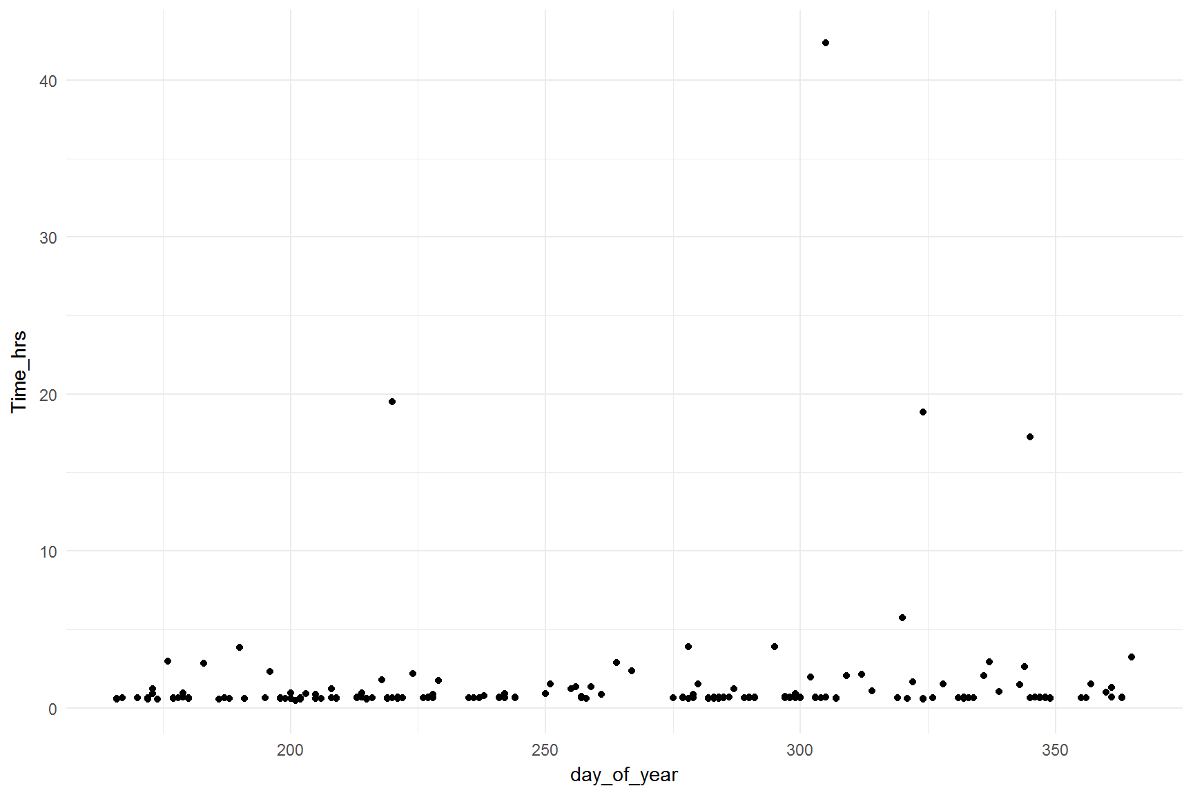
I did not do any 40+ hour rides. These outliers are due to me pausing a ride, leaving the bike overnight, and then riding the next day or several days later. This resulted in a single ride on one file with a very long elapsed time (which is different than riding time, but my Google spreadsheet did not report that apparently). The elapsed time is therefore misleading, as it is not riding time.
Examine distributions of distances
Since the elapsed time could be misleading, I will instead focus on distance.
# set order of days of week
rides_df$day_name <- factor(rides_df$day_name, levels =
        c("Mon", "Tue", "Wed", "Thu", "Fri", "Sat", "Sun"))

# density plots
density_plot1 <- rides_df %>%
        ggplot(aes(x = distance_miles, y = day_name, fill = ..x..)) +
        geom_density_ridges_gradient() +
        scale_fill_viridis(name = "distance", option = "D") +
        labs(title = "Distribution of Distance Ridden Given the Day of the Week",
             x = "Miles", y = "") +
        theme_minimal()

density_plot2 <- rides_df %>%
        ggplot(aes(x = distance_miles, y = month, fill = ..x..)) +
        geom_density_ridges_gradient() +
        scale_fill_viridis(name = "distance", option = "D") +
        labs(title = "Distribution of Distance Ridden Over Each Month",
             x = "Miles", y = "") +
        theme_minimal()
density_plot1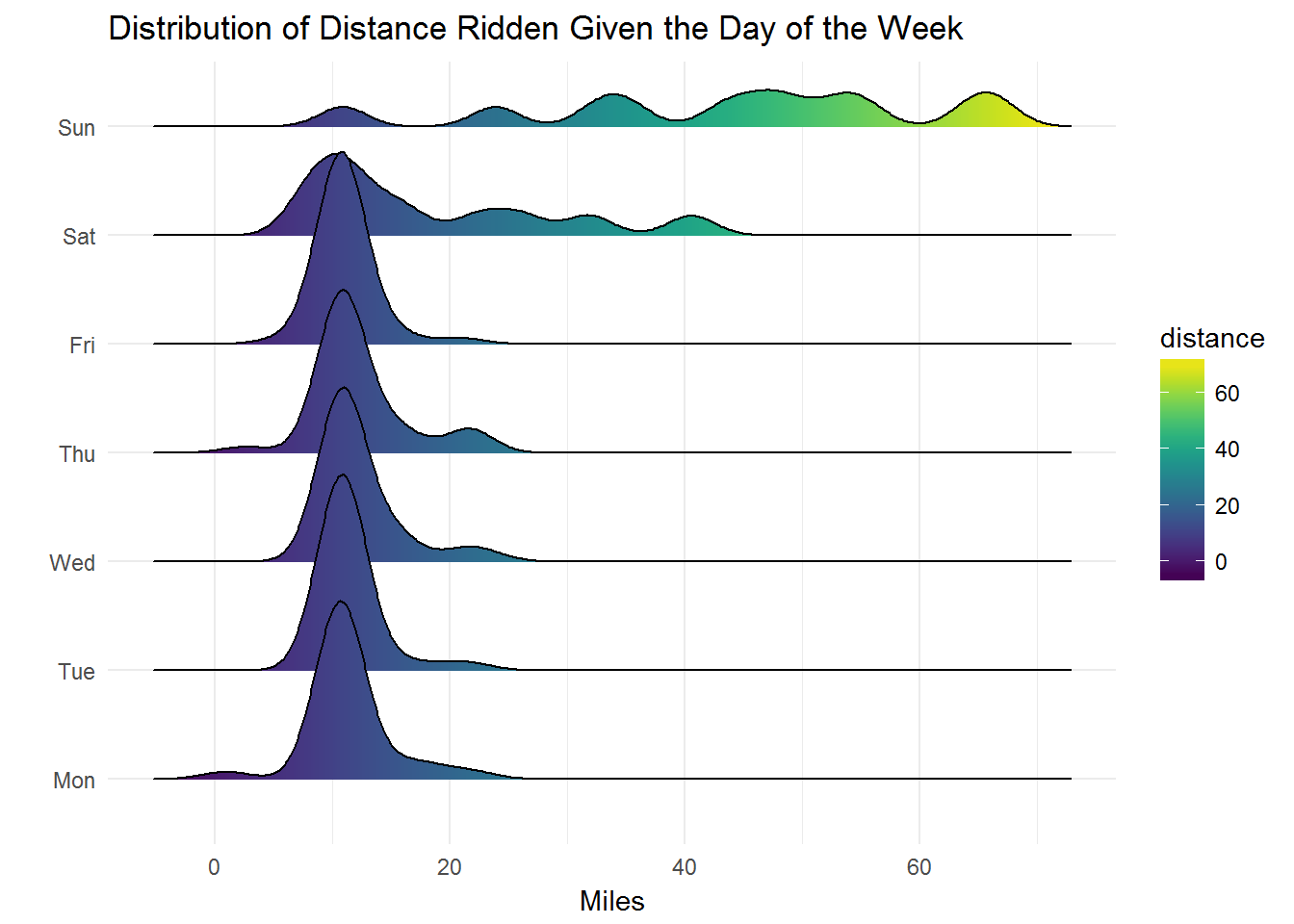
density_plot2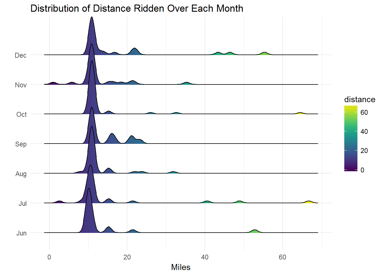
It is likely unsurprising that I tend to ride longer on weekends than weekdays. Most of my weekdays cluster at 11 miles, which is the length of my commute to and from work. This pattern holds true for each month as well. The majority of my rides are 11 miles.
Finally, I’ll make several different types of plots and then join these into one summary figure. I want to get a quick glance of how far I tend to ride depending on the day and month and my progress over time compared to my goal of 4000 miles.
# scatter plot
rides_scatter <- rides_df %>%
        ggplot(aes(x = day_of_year, y = distance_miles, color = day_name)) +
        geom_point() +
        scale_color_viridis(discrete = TRUE, option = "D") +
        theme_minimal(base_size = 12) +
        labs(x = "Day of Year",
             y = "Distance (miles)",
             title = "Distance by Day of Year") +
        guides(fill=FALSE) # remove legend

#----------------------------------------------------------------------------
# distance by day and month
rides_day_dst <- rides_df %>%
        ggplot(aes(x = factor(month), y = distance_miles, fill = day_name)) +
        geom_bar(stat = "identity", width = 0.9) +
        scale_fill_viridis(discrete = TRUE) +
        theme_minimal(base_size = 12) +
        labs(x = "Month",
             y = "Distance (miles)",
             title = "Distance by Day and Month")

# order factors for day name
rides_df3$day_name <- factor(rides_df3$day_name, levels =
        c("Mon", "Tue", "Wed", "Thu", "Fri", "Sat", "Sun"))

# percentage plot - not showing for now
rides_day_dst_perc <- rides_df3 %>%
        ggplot(aes(x = factor(month), y = perc*100, fill = day_name)) +
        geom_bar(stat="identity", width = 0.9) +
        theme_minimal(base_size = 12) +
        scale_fill_viridis(discrete = TRUE) +
         labs(x = "Month",
             y = "Percent Distance",
             title = "Percent Distance by Day and Month")

#-----------------------------------------------------------------------------
# cumulative distance compared to goal. first set order.
rides_df2$day_name <- factor(rides_df2$day_name, levels =
        c("Mon", "Tue", "Wed", "Thu", "Fri", "Sat", "Sun"))

rides_4k <- rides_df2 %>%
        filter(day_of_year >=165) %>%
        ggplot(aes(x = day_of_year, y = cumsum(distance_miles))) +
        # geom_bar(stat = "identity") +
        geom_point(aes(color = day_name)) +
        geom_line(aes(x = day_of_year, y = cumsum(daily_distance_goal_4k))) +
        scale_color_viridis(discrete = TRUE) +
        guides(fill=FALSE) +
        theme_minimal(base_size = 12) +
        labs(x = "Day of Year",
             y = "Cumulative distance (miles)",
             title = "Accumulated vs 4000 Mile Yearly Goal")

#--------------------------------------------------------------------------------
Summary of cycling for the second half of 2017
#output the visualizations using ggarrange:
ggarrange(rides_scatter, rides_4k, rides_day_dst,
          labels = c("", "", "", ""),
          common.legend = TRUE, # make a common legend since all color is Day Name
          legend = "right",
          ncol = 1, nrow = 3)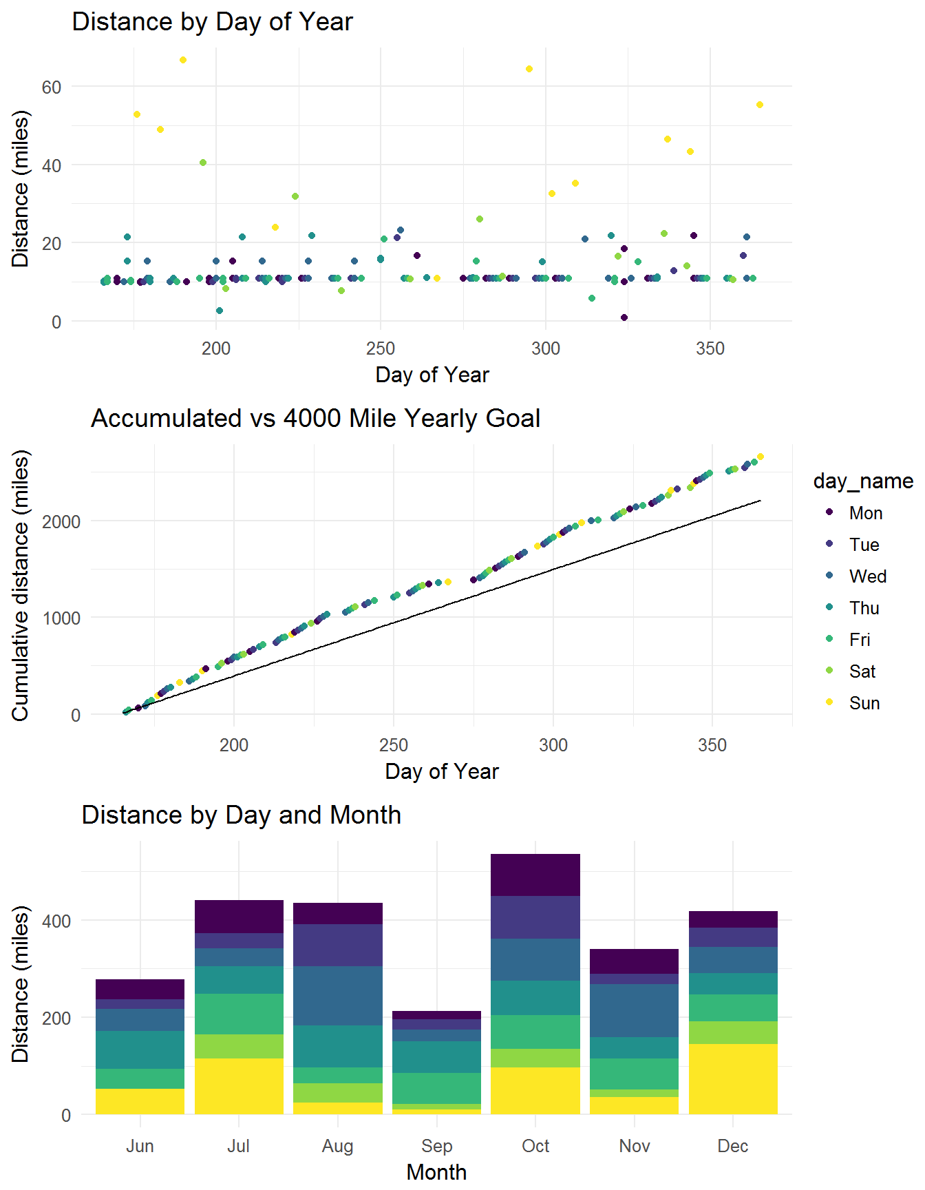
My longer rides tend to be on Sunday, while most of my rides during the weekday are 11 miles. For the portion of the year examined, I exceeded my 4000 mile goal (however, injury during the first part of the year meant I actually did not achieve 4000 miles). The bottom graph lets me examine my monthly distance, and which days were responsible for the distance. I travelled a lot in September, and started riding more on Sunday in December.